Base Learners

Mathematical notation

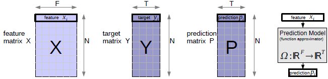
Bold faced symbols (X,Y,x...) are used for vectors and matrices, non-bold for scalars. In Figure 1 there is an overview of the data matrices. We use a multiple feature/input and multiple target/output notation, which is dedicated to cover the high dimensional input and output space. The data matrix is X, a NxF matrix with elements x_ij, where N is the number of training examples and F is the size of the input (input dimensionality). x_ij is the j-th feature of sample i. The rows of X are the input features. Target values y_ij are denoted as matrix Y of size NxT, where T is the number of target values (output dimensionality). y_ij is the j-th target value of sample i. Each single target is a row in Y. Predictions p_ij are denoted as matrix P of size NxT. Any learner uses X and Y P. The prediction model is Ω : ℝ ^F↦ℝ^T, which represents the function approximation from input to output space. When working with classification problems, C is the number of classes, the corresponding encoded target vectors y_i are C-dimensional with labels l_i. We use the value of +1 to encode class labels and -1 for other values in y_i.

When we view the data in form of a list, we use L={(x₁,y₁)...(x_N,y_N)} as notation for the training set. Each sample is a tuple of the feature vector and the target. This is typical for gradient descent based algorithms, where the training is done epoch-wise, in one particular epoch example-wise.

Data Normalization

Linear Regression - LR

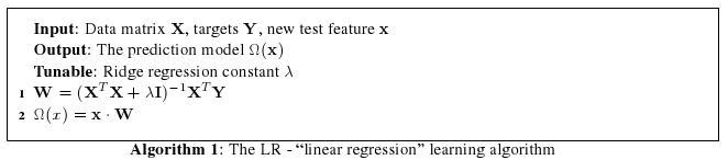
A linear regression model predicts new input samples by a linear combination of input features with weights W. The weights are denoted by a FxT matrix, so new inputs x (row vectors) are predicted by

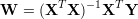
Estimation of the weights can be done by gradient descent, but a linear solver is more efficient. Linear combination weights can be obtained by evaluating the following expression. The matrix X is the data set (features) and Y the target values.

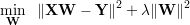
One can penalize large weights by modifying the loss function with L2-regularization of the weights, this is also known as “weight-decay”. Following function needs to be minimized with respect to W. When we apply the norm ||⋅|| to a matrix, we take the frobenius norm ||A||_F=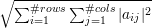

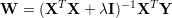
The next equation is the closed solution to this minimization problem.

The identity matrix is denoted by I and λ is the ridge regression constant (or Tikhonov regularization. The regularizer λ controls the smallest eigenvalues of X^TX, thus the magnitudes of the weights W shrinks with higher values of λ. In our software implementation we multiply the constant λ by the number of equations N. Please note that no constant 1 input is provided here, the features should contain a constant 1 column.

Polynomial Regression - PR

Polynomial regression is linear regression with a non-linear transformation on the input features. This means the training features x are enlarged by the help of a binomial series (1 + x)^α.

The number of terms, in the case of adding all cross interactions to augment the feature set is F ⋅ (F + 1)∕2 when having a degree-2 polynomial. It is clear that this only works for a small number of features. We are going to use the shortcut “poly2” for a polynomial regression with degree 2 and no cross-terms. “poly2-cross” is the same as poly2 but with all cross interaction terms.

Neural Networks - NN

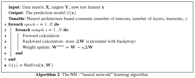
Artificial neural networks are functions approximators, based on simple computational units, called neurons. The model was developed in the 70’ and is somewhat "brain-inspired" where biological neurons aggregate weighted inputs to produce a non-linear output. In biology, neural nets use spikes (small electric impulses), artificial neural networks operate in the real-valued domain. The net is built of single neurons, connected together via weights. The structure can be defined by the designer, but in general it is layer oriented. This enables a more structured view on the arrangement of neurons and a net structure can be fully described by the number of hidden layers and the number of neurons in each layer. Learning is typically done with gradient descent.

In the past, neural networks have beed used in many applications, such as handwritten digit recognition, email spam detection, financial prediction, biometrics, image recognition and feature extraction. They often outperform simple methods like linear regression or k-nearest neighbors methods and compare well to SVMs. One of the big advantages of neural networks is that all learned knowledge is encoded in the weights, this makes the prediction very fast.

The internal modeling of the data, found by the weights, are hard to interpret. All learned information, during training a Neural Network, are encoded in its weights. An artificial neural network can model complex interactions within the data and has no problem in handling collinear inputs. The output is bounded by the activation function of the output layer. But it is also possible to place linear output units for prediction.

An alternative usage of a neural networks is the training of an autoencoder. An autoencoder is a layer-symmetric net (with one coding layer in the middle), the goal is to perform non-linear dimensionality reduction. In this type of network architecture, the inputs should be equal to the outputs, the idea is to reconstruct the output by passing the data through a bottleneck layer. The low-dimensional code in the middle layer can be used as new dimensionality-reduced features. There exists a computational efficient algorithm to train neural networks, the backpropagation algorithm. We wont go into the details of the backpropagation algorithm because it is well known in machine learning.

When training a classification task, where the targets have values of -1 and +1, it is not optimal to place a tanh unit at the output layer. The tanh unit has an output swing of -1 to +1, thus it will never approximate the targets with zero error because the targets are placed to the asymtotes of the tanh function. Based on many experiments on the MNIST and UCI data sets we found a simple output mapping, which suggests to muliply the output of the tanh unit with 1.2. This keeps the non-linearity and enables the net to cover the output range.

K-Nearest Neighbors - KNN

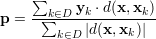
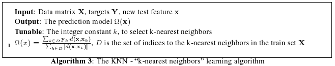
Finding k-nearest neighbors in the feature space is one of the oldest machine learning algorithms. The algorithm is instance-based and uses a distance metric (e.g. euclidean distance) to find k-nearest training samples to the one, which is going to be predicted. For regression, the prediction of a new test feature x is generated by a weighted sum over k-nearest targets y in the training set. The KNN requires no training, on every new prediction, the algorithm must search through the whole training set to find best neighbors. The algorithm is very strong when distances are well defined. The following formula is used to predict a test feature x. The k-nearest neighbors algorithm is a popular approach in collaborative filtering, the prediction accuracy can be improved by applying a non-linear envelop (e.g. sigmoid function) over the distances d(x,x_k). We also tried to wrap a sigmoid function around the distances, but we observed no improvement. The prediction vector is given by

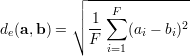
The set D consists of indices of the k-nearest Neighbors to x in the training samples, y_k are the corresponding target vectors in the training set. This means we calculate the distances to the input features and select the largest k. The distance metric d(a,b) is used to compare two feature vectors and find the k-nearest neighbors in the feature space ℝ^F. The whole prediction formula is a weighted average of k targets in the training set, hence the name "instance based" learner. Since the distance measure can have negative values (e.g. Pearson correlation), the denominator is the sum of absolute distances. A popular distance metric is the euclidean distance d_e(a,b), the following formula is the definition of the euclidean distance between two feature vectors a and b.

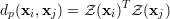
another distance measure is the Pearson correlation coefficient, given by

where Z(x) denotes the z-score of the vector x. The z-score is calculated by centering the values in x around its mean and scale it to standard deviation to 1. The advantage of the Pearson correlation is that the distance is calculated by a dot product of z-normalized input features. This can be done very efficiently by matrix-matrix multiplication. The euclidean distance can also be computed efficiently using matrix-matrix multiplication routines.

In order to find the closest match we use the inverse of the euclidean distance d(x_i,x_j)= distance metric, it works well in our experiments. The inverse function is necessary, because we are selecting the k-largest distances in the feature space. The number of 0.01 in the denominator makes the inverse stable for small values of d_e. This forms the set D, the indices to the k-nearest neighbors.

K-nearest neighbors models have quadratic prediction time O(N²), where N is the number of training samples, which is not suitable for generating fast predictions (in the case of a large training set). On the other hand, no training is required.

Kernel Ridge Regression - KRR

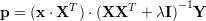
Linear regression can be viewed in a dual representation. Where standard linear regression needs dot products of input dimensions (columns of data matrix X), kernel ridge regression relies on dot product of input features (rows of data matrix X). If a linear kernel k(a,b)=a^Tb is used, KRR is equivalent to linear regression. Recall the prediction of a linear regression is p=xW. Where the linear weights are calculated by W=(X^TX+λX)^-1X^TY. Now we can reformulate the prediction formula

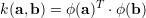
The matrix G=XX^T is called the "gram matrix", it contains all dot products of input features and is symmetric. Also the first term xX^T are dot products of the new input feature with the training set A. Therefore we can kernelize the dot products by defining a mapping ϕ(x) to a high dimensional space

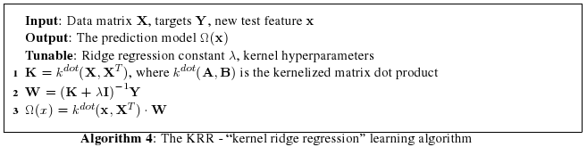
We experimented with few different kernels, the following two kernels are most successful. The first is the polynomial kernel k(a,b)=(α a^Tb+β)^p and the gauss kernel (or RBF kernel) k(a,b)=exp(-). We use the notation of k^dot(A,B) to denote the kernelized matrix-matrix product. This means that on each point of the target matrix, the dot product gets calculated with the current kernel. The computational and memory intensive step is the inverse of the Gram matrix (K+λI)^-1, which time complexity is O(N³). This limits the number of training samples to around 60000, when using KRR as learn algorithm (assuming single precision an a 16GB machine (2.)).

Gradient Boosted Decision Trees - GBDT

The shortcut "GBDT" is associated with many great ideas. We will explain them in this section. First, this learning algorithm comes from the family of trees. A decision tree consists of nodes and leafs. A single tree has one root node, this is the starting point of the algorithm. When the tree makes a prediction, it compares a certain feature x_i of the feature vector x with a threshold θ. If the feature is larger than θ, the algorithm continues recursively with the left subtree, else with the right subtree. When a leaf is a termination node, the prediction is a constant value (in most trees). The constant can be the average of the targets from the train samples reching this termination node. A decision tree uses axis-parallel splits to slice and dice the feature space. We can now summarize, a node stores a threshold θ, an index i to the feature x_i and two pointers to a left and a right subtree (again nodes). A leaf stores a constant (the prediction) and is itself a termination node. The challenge of training a decision tree is to find good split values θ and good corresponding single feature indices i. We use a greedy algorithm to train the decision tree, which uses the best split in terms of reducing the RMSE after each split. One tree is trained for every target. Begin with the root node, where the training algorithm has access to all input features. The first split is the one that reduces the RMSE best when predicting two constant values. The next node for the next split is choosen as the one with the most training samples. The process of spliting is stopped when one of the following criterias is met. First, no split improves the RMSE on the training set. Second the maximum number of splits are reached. Or third, when the number of training examples, which are passed through the tree, has a size less than 2 (too less data available).

A tree alone has several disadvantages. For instance, axis-parallel splits can not model a smooth function, the prediction is a constant for some regions of the input space. The tree is known to easily overfit the data. And it is prone to have an unstable behavior, small changes in the train data can lead to total different trees. Breiman has published a useful idea in 2001, the name of the paper was "Random Forests" [..]. The core idea is to limit the number of feature candidates in finding the optimal split per node. Per node, a new random subspace of features is generated. A good empirical value is starting with a random subset of features taking in consideration to find the optimal split. No pruning is used here. This modification leads to better generalization behavior, in other words lower error on the test set.

Gradient boosting is an idea from Friedman [..], [..] and has a distinctive relation to training on residuals (an ensemble learning method). The algorithm runs epoch-wise, in each epoch the learner is trained on the residuals of the outcomes from all previous learners. In the first epoch the targets Y₁ are the original residuals, the learner's prediction is P. In the second epoch, the targets are Y₂=Y₁-ηP₁. In the third epoch, the targets are Y₃=Y₁-ηP₁-ηP₂. This means that only a part of the learned model is subtracted from the targets. Hence the name "gradient" because gradient boosting appoaches the target with the gradient of the learner’s prediction. The learning rate η controls how much of the predictions are subtracted by the targets, this mechanism results in learning only a fraction of the data in one epoch. The learning curve can be compared to neural network, where after some epochs the gradient boosted decision tree begins to overfit. This is the point to stop training (early stopping mechanism). Typical values for η are 0.1. The final effect of gradient boosting applied to learning decision trees is to smooth the predictions.

Both ideas, random forests and gradient boosting improves the accuracy and generalization ability of the decision tree as base learner. This has the drawback of longer training and prediction time.